Mathematical art (beyond Lissajous)
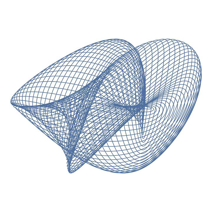
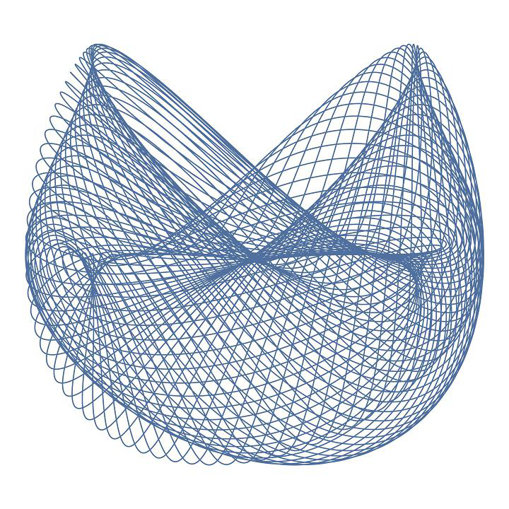
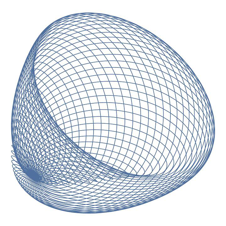
Sure, Lissajous plots are useful. In electronics they may help you find the phase between two (sinusoidal) signals, for instance, but they get boring quickly. I wrote a Mathematica program to create other parametric plots, still based on just sums and products of sines. The results are sometimes amazing, as you can see in the examples below. Each image is accompanied with the set of equations that generated it.
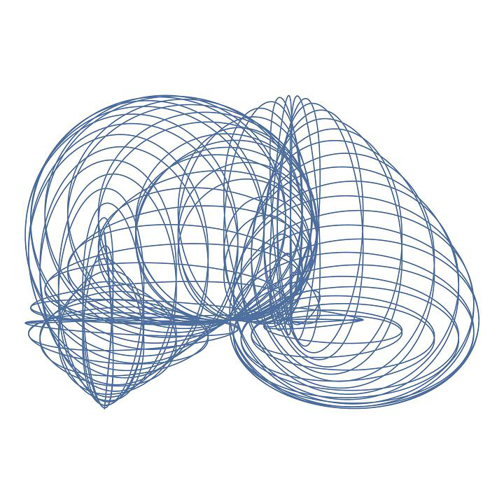
$$ \begin{cases} x(t) = cos(3 t) \cdot cos(79 t) + sin(2 t) \\[1em] y(t) = sin(2 t + \dfrac{\pi}{4}) \cdot ( sin(79 t) + sin(2 t)) \end{cases} $$
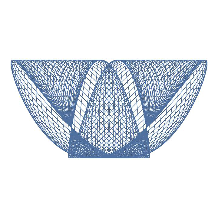
$$ \begin{cases} x(t) = sin(53 t) \cdot sin(54 t + \dfrac{\pi}{4}) + sin(53 t + \dfrac{\pi}{4}) \\[1em] y(t) = sin(53 t + \dfrac{\pi}{4}) \cdot \left( sin(53 t) + sin(53 t + \dfrac{\pi}{4}) \right) \end{cases} $$
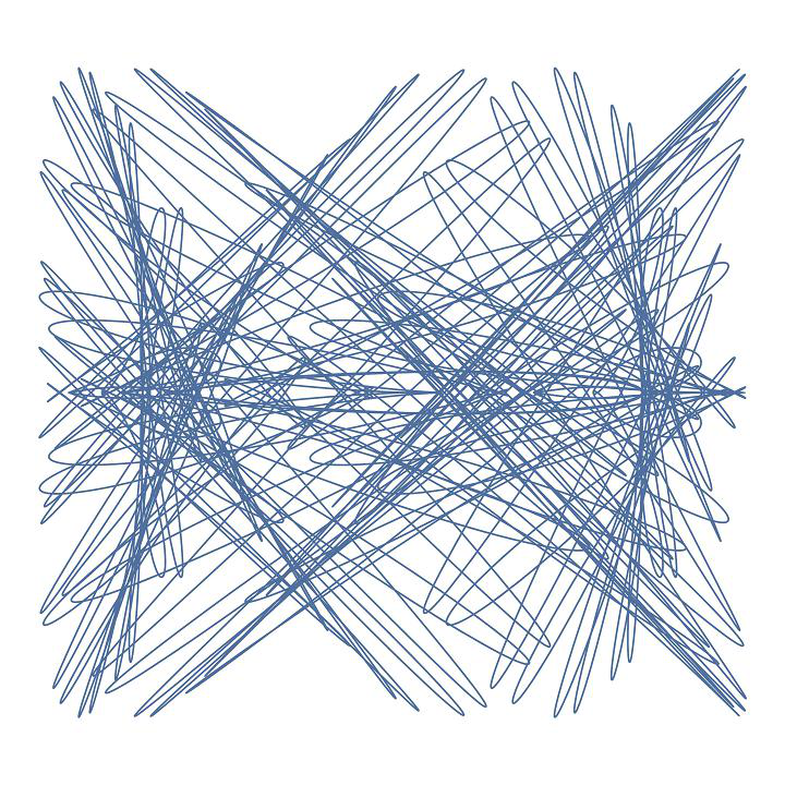
$$ \begin{cases} x(t) = sin(3 t) + cos(3 t) \cdot cos(97 t) \\[1em] y(t) = sin(5 t) \cdot \left( cos(5 t) + cos(97 t) \right) \end{cases} $$
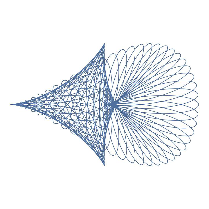
$$ \begin{cases} x(t) = sin(7 t) \cdot \left( 1 + sin(59 t) \right) \\[1em] y(t) = cos(7 t) \cdot \left( sin(7 t) + sin(59 t) \right) \end{cases} $$
$$ \begin{cases} x(t) = cos(53 t) + sin(31 t + \dfrac{\pi}{4}) \cdot sin(53 t + \dfrac{\pi}{4}) \\[1em] y(t) = \left(sin(53 t + \dfrac{\pi}{4})\right)^2 + cos(31 t) \cdot sin(53 t) \end{cases} $$
$$ \begin{cases} x(t) = sin(61 t) + cos(61 t) \cdot cos(37 t) \\[1em] y(t) = \left( sin(61 t) \right)^2 + sin(37 t) \cdot sin(61 t + \dfrac{\pi}{4}) \end{cases} $$
$$ \begin{cases} x(t) = sin(71 t) \cdot \left(sin(71 t) + cos(11 t) \right) \\[1em] y(t) = \dfrac{1}{2} \cdot cos(30 t) \cdot \left( (\sqrt{2}+1) \cdot cos(71 t) + sin(71 t) \right) \cdot \left( cos(41 t) + sin(41 t) \right) \end{cases} $$